
In this case there are no simple
equations we can use at this level. If the equation of the motion is known then calculations
can be carried out.
However problems of non-uniform acceleration can be solved by
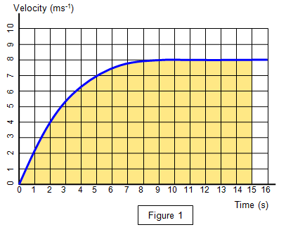
using graphical methods. One example is the 100m sprint shown below. (Figure 1)
This
example of non-uniform acceleration provides a useful practical example of velocity time
graphs.
The graph in Figure 1 shows how the velocity of a schoolgirl sprinter
varies with time during a 100 m race. Notice that she accelerates rapidly at the start, the
graph is steep, and then reaches a constant velocity after about 8s. The shaded area
represents a distance of 100m and so she took 15 s to complete the
race.
The gradient of the line at any point gives the instantaneous acceleration at that point.
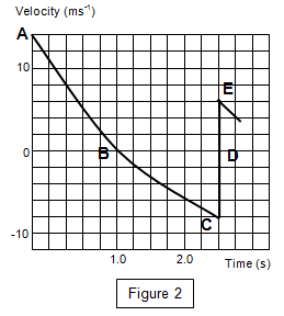 A light rubber ball is thrown vertically upwards at 14 ms-1 and Figure 2 represents the velocity-time graph for part of the resulting motion.
(a) Describe the motion briefly.
A light rubber ball is thrown vertically upwards at 14 ms-1 and Figure 2 represents the velocity-time graph for part of the resulting motion.
(a) Describe the motion briefly.